In-class Exercise 2: Spatial Point Patterns Analysis: spatstat methods
21 Jul 2025
Issue 1: Installing maptools
After the installation is completed, it is important to edit the code chunk as shown below in order to avoid maptools being download and install repetitively every time the Quarto document been rendered.

Working with st_union()
Creating ppp objects from sf data.frame
Instead of using the two steps approaches discussed in Hands-on Exercise 3 to create the ppp objects, in this section you will learn how to work with sf data.frame.
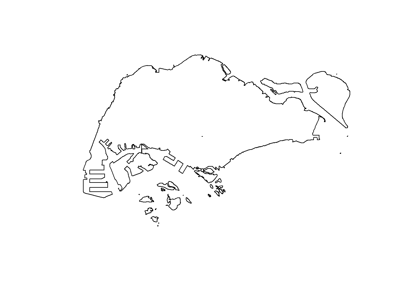
In the code chunk below, as.ppp() of spatstat.geom package is used to derive an ppp object layer directly from a sf tibble data.frame.
Warning in default.charmap(ntypes, chars): Too many types to display every type
as a different character
Warning in default.charmap(ntypes, chars): Too many types to display every type
as a different character
Warning in default.charmap(ntypes, chars): Too many types to display every type
as a different character
Warning in default.charmap(ntypes, chars): Too many types to display every type
as a different character
Warning in default.charmap(ntypes, chars): Too many types to display every type
as a different character
Warning: Only 10 out of 1925 symbols are shown in the symbol mapWarning in default.charmap(ntypes, chars): Too many types to display every type
as a different characterWarning: Only 10 out of 1925 symbols are shown in the symbol map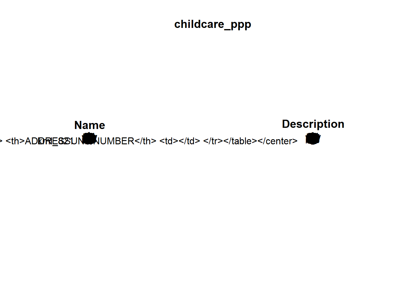
Next, summary() can be used to reveal the properties of the newly created ppp objects.
Marked planar point pattern: 1925 points
Average intensity 2.417323e-06 points per square unit
Coordinates are given to 11 decimal places
Mark variables: Name, Description
Summary:
Name Description
Length:1925 Length:1925
Class :character Class :character
Mode :character Mode :character
Window: rectangle = [11810.03, 45404.24] x [25596.33, 49300.88] units
(33590 x 23700 units)
Window area = 796335000 square unitsCreating owin object from sf data.frame
In the code chunk as.owin() of spatstat.geom is used to create an owin object class from polygon sf tibble data.frame.
Next, summary() function is used to display the summary information of the owin object class.
Window: polygonal boundary
80 separate polygons (35 holes)
vertices area relative.area
polygon 1 14650 6.97996e+08 8.93e-01
polygon 2 (hole) 3 -2.21090e+00 -2.83e-09
polygon 3 285 1.61128e+06 2.06e-03
polygon 4 (hole) 3 -2.05920e-03 -2.63e-12
polygon 5 (hole) 3 -8.83647e-03 -1.13e-11
polygon 6 668 5.40368e+07 6.91e-02
polygon 7 44 2.26577e+03 2.90e-06
polygon 8 27 1.50315e+04 1.92e-05
polygon 9 711 1.28815e+07 1.65e-02
polygon 10 (hole) 36 -4.01660e+04 -5.14e-05
polygon 11 (hole) 317 -5.11280e+04 -6.54e-05
polygon 12 (hole) 3 -3.41405e-01 -4.37e-10
polygon 13 (hole) 3 -2.89050e-05 -3.70e-14
polygon 14 77 3.29939e+05 4.22e-04
polygon 15 30 2.80002e+04 3.58e-05
polygon 16 (hole) 3 -2.83151e-01 -3.62e-10
polygon 17 71 8.18750e+03 1.05e-05
polygon 18 (hole) 3 -1.68316e-04 -2.15e-13
polygon 19 (hole) 36 -7.79904e+03 -9.97e-06
polygon 20 (hole) 4 -2.05611e-02 -2.63e-11
polygon 21 (hole) 3 -2.18000e-06 -2.79e-15
polygon 22 (hole) 3 -3.65501e-03 -4.67e-12
polygon 23 (hole) 3 -4.95057e-02 -6.33e-11
polygon 24 (hole) 3 -3.99521e-02 -5.11e-11
polygon 25 (hole) 3 -6.62377e-01 -8.47e-10
polygon 26 (hole) 3 -2.09065e-03 -2.67e-12
polygon 27 91 1.49663e+04 1.91e-05
polygon 28 (hole) 26 -1.25665e+03 -1.61e-06
polygon 29 (hole) 349 -1.21433e+03 -1.55e-06
polygon 30 (hole) 20 -4.39069e+00 -5.62e-09
polygon 31 (hole) 48 -1.38338e+02 -1.77e-07
polygon 32 (hole) 28 -1.99862e+01 -2.56e-08
polygon 33 40 1.38607e+04 1.77e-05
polygon 34 (hole) 40 -6.00381e+03 -7.68e-06
polygon 35 (hole) 7 -1.40545e-01 -1.80e-10
polygon 36 (hole) 12 -8.36709e+01 -1.07e-07
polygon 37 45 2.51218e+03 3.21e-06
polygon 38 142 3.22293e+03 4.12e-06
polygon 39 148 3.10395e+03 3.97e-06
polygon 40 75 1.73526e+04 2.22e-05
polygon 41 83 5.28920e+03 6.76e-06
polygon 42 211 4.70521e+05 6.02e-04
polygon 43 106 3.04104e+03 3.89e-06
polygon 44 266 1.50631e+06 1.93e-03
polygon 45 71 5.63061e+03 7.20e-06
polygon 46 10 1.99717e+02 2.55e-07
polygon 47 478 2.06120e+06 2.64e-03
polygon 48 155 2.67502e+05 3.42e-04
polygon 49 1027 1.27782e+06 1.63e-03
polygon 50 (hole) 3 -1.16959e-03 -1.50e-12
polygon 51 65 8.42861e+04 1.08e-04
polygon 52 47 3.82087e+04 4.89e-05
polygon 53 6 4.50259e+02 5.76e-07
polygon 54 132 9.53357e+04 1.22e-04
polygon 55 (hole) 3 -3.23310e-04 -4.13e-13
polygon 56 4 2.69313e+02 3.44e-07
polygon 57 (hole) 3 -1.46474e-03 -1.87e-12
polygon 58 1045 4.44510e+06 5.68e-03
polygon 59 22 6.74651e+03 8.63e-06
polygon 60 64 3.43149e+04 4.39e-05
polygon 61 (hole) 3 -1.98390e-03 -2.54e-12
polygon 62 (hole) 4 -1.13774e-02 -1.46e-11
polygon 63 14 5.86546e+03 7.50e-06
polygon 64 95 5.96187e+04 7.62e-05
polygon 65 (hole) 4 -1.86410e-02 -2.38e-11
polygon 66 (hole) 3 -5.12482e-03 -6.55e-12
polygon 67 (hole) 3 -1.96410e-03 -2.51e-12
polygon 68 (hole) 3 -5.55856e-03 -7.11e-12
polygon 69 234 2.08755e+06 2.67e-03
polygon 70 10 4.90942e+02 6.28e-07
polygon 71 234 4.72886e+05 6.05e-04
polygon 72 (hole) 13 -3.91907e+02 -5.01e-07
polygon 73 15 4.03300e+04 5.16e-05
polygon 74 227 1.10308e+06 1.41e-03
polygon 75 10 6.60195e+03 8.44e-06
polygon 76 19 3.09221e+04 3.95e-05
polygon 77 145 9.61782e+05 1.23e-03
polygon 78 30 4.28933e+03 5.49e-06
polygon 79 37 1.29481e+04 1.66e-05
polygon 80 4 9.47108e+01 1.21e-07
enclosing rectangle: [2667.54, 56396.44] x [15748.72, 50256.33] units
(53730 x 34510 units)
Window area = 781945000 square units
Fraction of frame area: 0.422Combining point events object and owin object
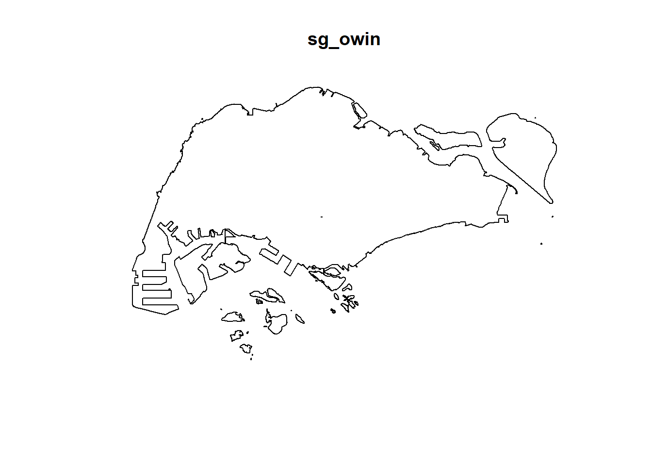
Using the step you learned from Hands-on Exercise 3, create an ppp object by combining childcare_ppp and sg_owin.
The output object combined both the point and polygon feature in one ppp object class as shown below.
Warning in default.charmap(ntypes, chars): Too many types to display every type
as a different character
Warning in default.charmap(ntypes, chars): Too many types to display every type
as a different character
Warning in default.charmap(ntypes, chars): Too many types to display every type
as a different character
Warning in default.charmap(ntypes, chars): Too many types to display every type
as a different character
Warning in default.charmap(ntypes, chars): Too many types to display every type
as a different characterWarning: Only 10 out of 1925 symbols are shown in the symbol mapWarning in default.charmap(ntypes, chars): Too many types to display every type
as a different characterWarning: Only 10 out of 1925 symbols are shown in the symbol map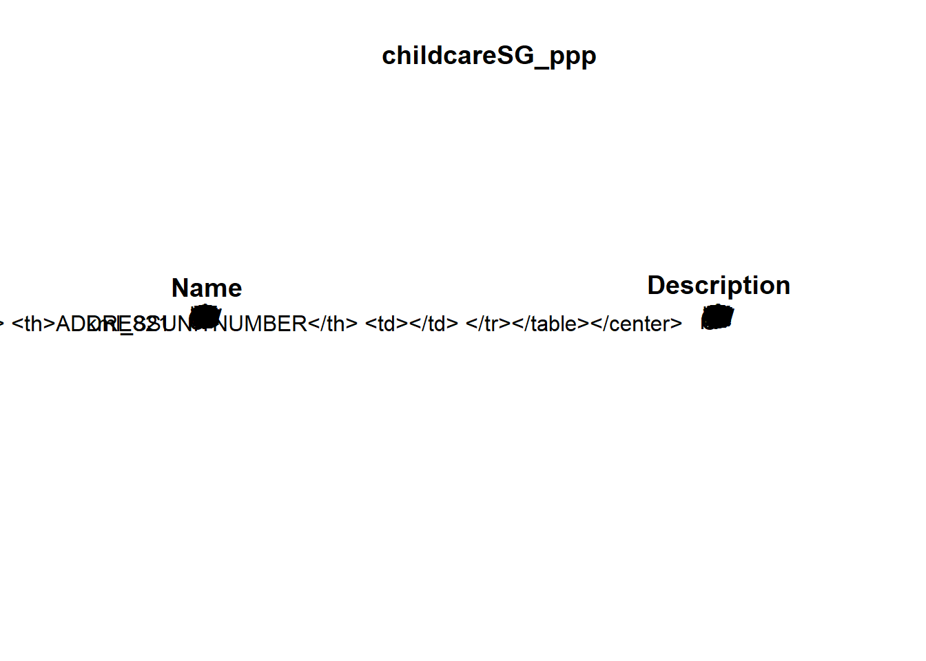
Kernel Density Estimation of Spatial Point Event
The code chunk below re-scale the unit of measurement from metre to kilometre before performing KDE.
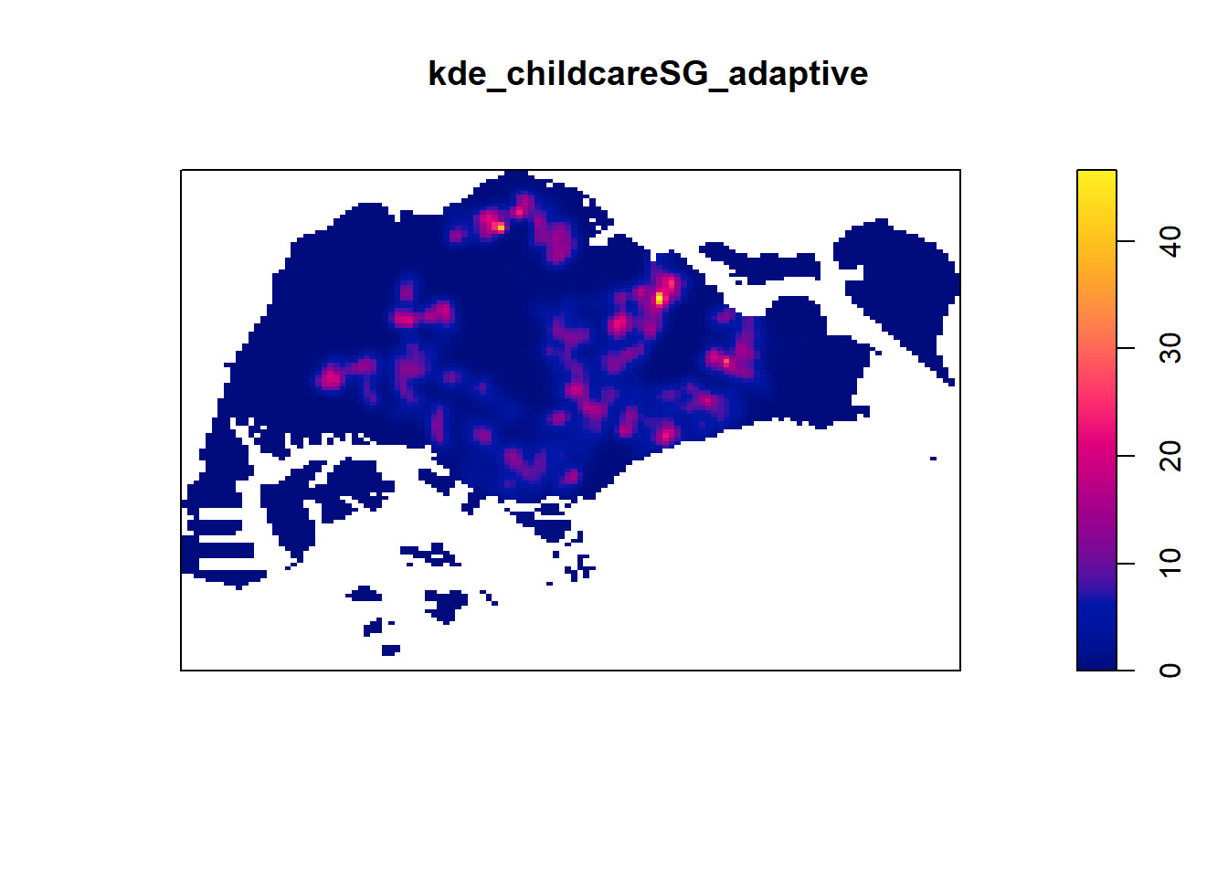
Kernel Density Estimation
Code chunk shown two different ways to convert KDE output into grid object
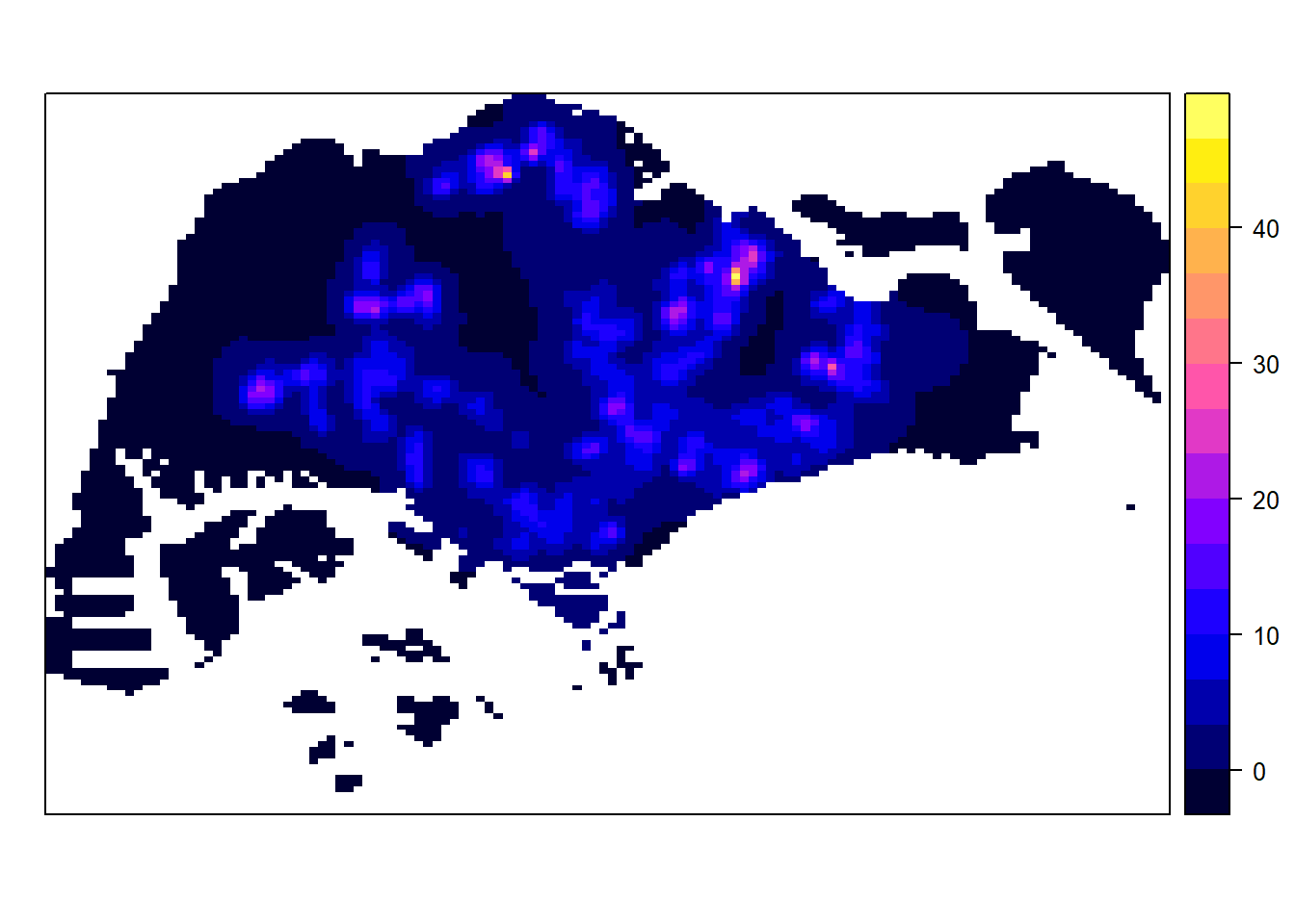
Kernel Density Estimation
Visualising KDE using tmap
The code chunk below is used to plot the output raster by using tmap functions.
tm_shape(kde_childcareSG_ad_raster) +
  tm_raster(palette = "viridis") +
  tm_layout(legend.position = c("right", "bottom"),
            frame = FALSE,
            bg.color = "#E4D5C9")
── tmap v3 code detected ───────────────────────────────────────────────────────[v3->v4] `tm_tm_raster()`: migrate the argument(s) related to the scale of the
visual variable `col` namely 'palette' (rename to 'values') to col.scale =
tm_scale(<HERE>).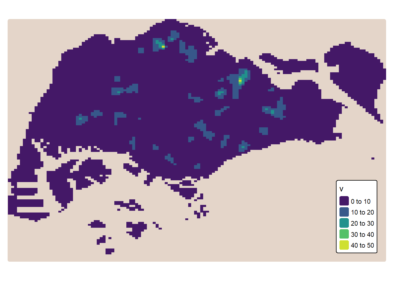
Extracting study area using sf objects
Extract and create an ppp object showing child care services and within Punggol Planning Area
On the other hand, filter() of dplyr package should be used to extract the target planning areas as shown in the code chunk below.
pg_owin <- mpsz_sf %>%
  filter(PLN_AREA_N == "PUNGGOL") %>%
  as.owin()

childcare_pg = childcare_ppp[pg_owin]

plot(childcare_pg)
Warning in default.charmap(ntypes, chars): Too many types to display every type
as a different character
Warning in default.charmap(ntypes, chars): Too many types to display every type
as a different character
Warning in default.charmap(ntypes, chars): Too many types to display every type
as a different character
Warning in default.charmap(ntypes, chars): Too many types to display every type
as a different character
Warning in default.charmap(ntypes, chars): Too many types to display every type
as a different characterWarning: Only 10 out of 72 symbols are shown in the symbol mapWarning in default.charmap(ntypes, chars): Too many types to display every type
as a different characterWarning: Only 10 out of 72 symbols are shown in the symbol map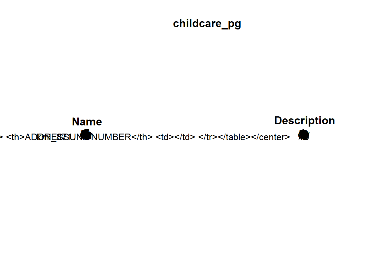
The Study Area
The study area is Bangkok Metropolitan Region.
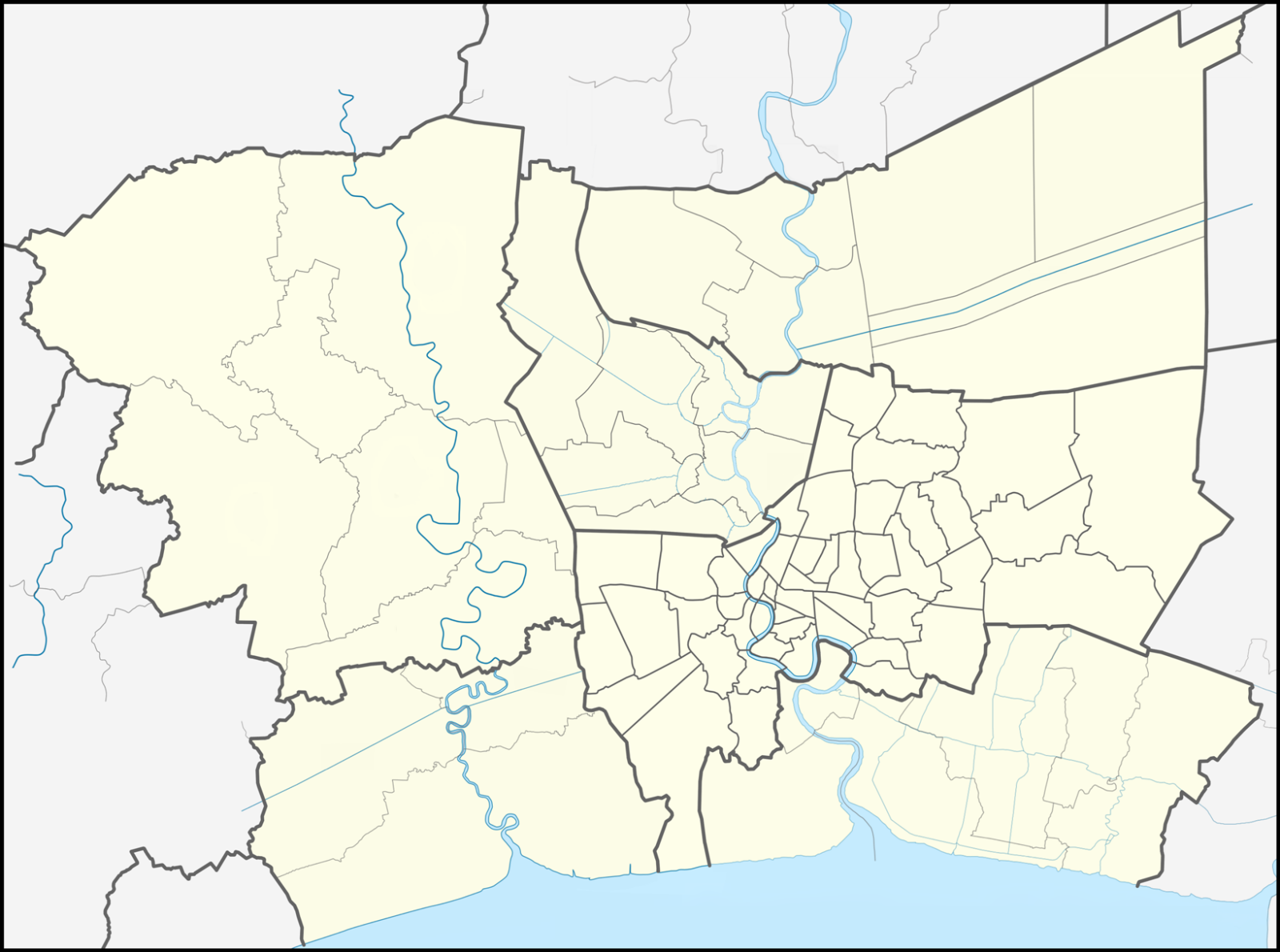
Note
The projected coordinate system of Thailand is WGS 84 / UTM zone 47N and the EPSG code is 32647.