In-class Exercise 3: Working with Open Government Data

Dr. Kam Tin Seong
Assoc. Professor of Information Systems(Practice)

School of Computing and Information Systems,
Singapore Management University

2025-09-11

Learning Outcome

By the end of this hands-on exercise, you will be able to:

• Preparing ACRA (Accounting and Corporate Regulatory Authority) Information on Corporate Entities datasets downloaded from data.gov.sg portal for geocoding,
• Geocoding the tidydata by using SLA OneMap API,
• Converting the geocoded transaction data into sf point feature data.frame, and
• Wrangling the sf point features to avoid overlapping point features.

Loading the R package

• The task
• The code

Write a code chunk to install and load tidyverse, sf, tmap and httr into R environment.

Note

• httr is an R package specially designed to provide a wrapper for the curl package, customised to the demands of modern web APIs. Key features: Functions for the most important http verbs: GET(), HEAD(), PATCH(), PUT(), DELETE() and POST().

• dplyr is a grammar of data manipulation, providing a consistent set of verbs that help you solve the most common data manipulation challenges. It is a must learned package for modern data scientists and data analysts. Refer to this chapter to learn more about dplyr.

• lubridate is an R package specially designed to handle date and date-time data type. Refer to this chapter to learn more about handle date and datetime with lubridate.

pacman::p_load(tidyverse, sf, tmap, httr)

Importing ACRA data

• The task
• The code

Write a code chunk to perform the followings:

• importing an ACRA data set into RStudio as tibble data frame, and
• drop the unnecessary fields such as fields with excessive missing values or fields with only single values.

folder_path <- "data/aspatial/acra"
file_list <- list.files(path = folder_path, 
                        pattern = "^ACRA*.*\\.csv$", 
                        full.names = TRUE)

acra_data <- file_list %>%
  map_dfr(read_csv)

Saving ACRA data

• The task
• The code

Write a code chunk to save the consolidated ACRA data.

write_rds(acra_data,
          "data/rds/acra_data.rds")

Tidying ACRA data

• The task
• The code

Write a code chunk to perform the followings:

• select the target businesses by using SSIC code,
• derive the year and month fields from registration_incorporation_date field,
• tidy postal code values to ensure avoid 5-digit postal codes by mistake, and
• select businesses registered in 2025.

biz_56111 <- acra_data %>%
  select(1:24) %>%
  filter(primary_ssic_code == 56111) %>%
  rename(date = registration_incorporation_date) %>%
  mutate(date = as.Date(date),
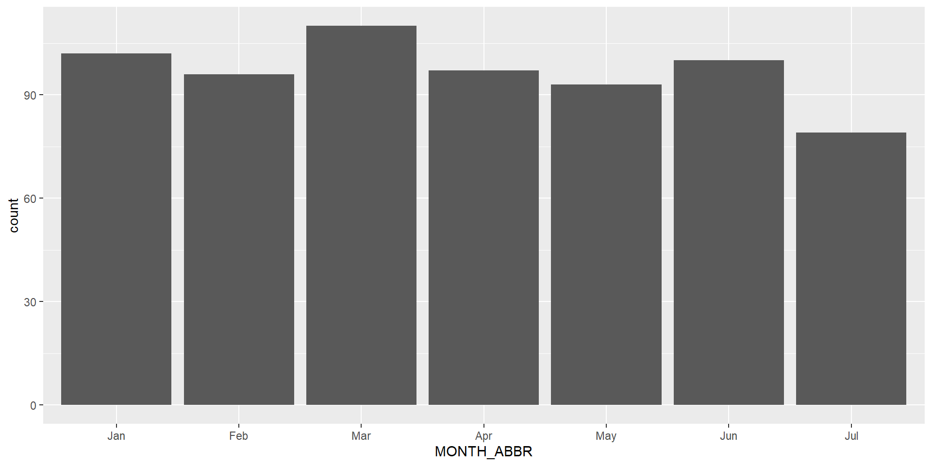
         YEAR = year(date),
         MONTH_NUM = month(date),
         MONTH_ABBR = month(date, 
                            label = TRUE, 
                            abbr = TRUE)) %>% 
  mutate(
    postal_code = str_pad(postal_code, 
    width = 6, side = "left", pad = "0")) %>%
           filter(YEAR == 2025)    

Geocoding

• The task
• The code

Write a function to perform the following tasks:

• Extracting unique postal code from the postal_code field of the tidied tibble data frame,
• performing geocode by submitting the postal codes to SLA OneMap Reverse Geocode API, and
• save the return results into two data frames namely found (for records that the postal codes are found) and not_found (for record that postal codes are not found).

postcodes <- unique(biz_56111$postal_code)

url <- "https://onemap.gov.sg/api/common/elastic/search"

found <- data.frame()
not_found <- data.frame(postcode = character())

for (pc in postcodes) {
  query <- list(
    searchVal = pc,
    returnGeom = "Y",
    getAddrDetails = "Y",
    pageNum = "1"
  )
  
  res <- GET(url, query = query)
  json <- content(res)
  
  if (json$found != 0) {
    df <- as.data.frame(json$results, stringsAsFactors = FALSE)
    df$input_postcode <- pc
    found <- bind_rows(found, df)
  } else {
    not_found <- bind_rows(not_found, data.frame(postcode = pc))
  }
}

Tidying the geocoded data

• The task
• The code

The geocoded data frame (i.e. found) contained many redundant fields. We only need the first ten fields. Write a code chunk to tidy the geocoded data frame.

found <- found %>%
  select(1:10)

Appending the location information

• The taks
• The code

Write a code chunk to append the location information (i.e. x- and y-coordinates) to biz_56111 sf data frame.

biz_56111 = biz_56111 %>%
  left_join(found, 
            by = c('postal_code' = 'POSTAL'))

Saving the data

• The task
• The code

Write a code chunk to save the tidied data into rds format for future use.

write_rds(biz_56111, "data/rds/biz_56111.rds")

Converting into SF data frame

• The Task
• The code

Write a code chunk to convert biz_56111 tibble data frame into sf data frame.

biz_56111_sf <- st_as_sf(biz_56111, 
                         coords = c("X","Y"),
                         crs=3414) 

Visualising the distribution

• The task
• The code

Write a code chunk to reveal the distribution of newly registered businesses by month.

ggplot(data = biz_56111,
       aes(x = MONTH_ABBR)) +
  geom_bar()

Visualising the business

• The Task
• The code

tmap_mode('view')
tm_shape(biz_56111_sf)+
  tm_dots()