Dr. Kam Tin Seong Assoc. Professor of Information Systems(Practice)
School of Computing and Information Systems, Singapore Management University
13 Sep 2025
Content
Introducing Spatial Point Patterns
The basic concepts of spatial point patterns
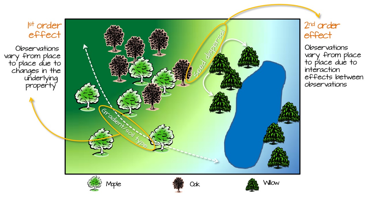
1st Order versus 2nd Order
Spatial Point Patterns in real world
1st Order Spatial Point Patterns Analysis
Quadrat analysis
Kernel density estimation
2nd Order Spatial Point Patterns Analysis
Nearest Neighbour Index
G-function
F-function
K-function
L-function
What is Spatial Point Patterns
Points as Events
Mapped pattern
Not a sample
Selection bias
Events are mapped, but non-events are not
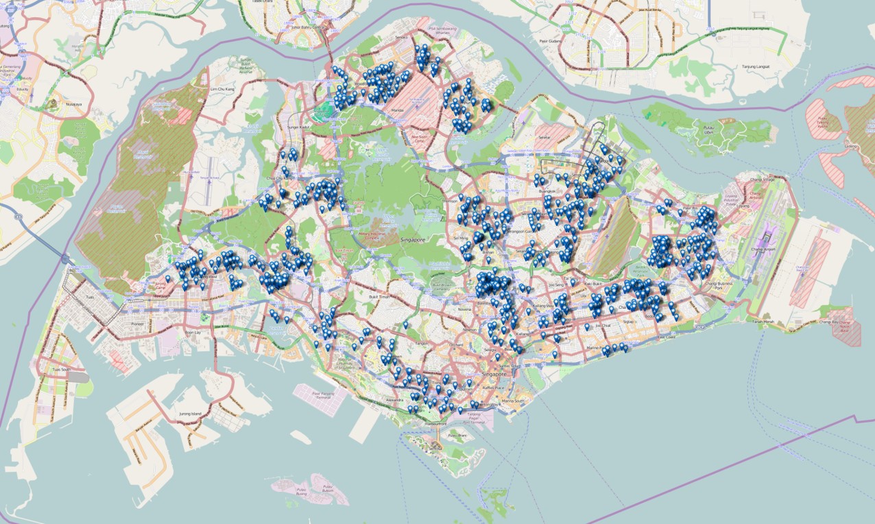
Spatial Point Patterns in Real World
Distribution of dieses such as dengue fever.
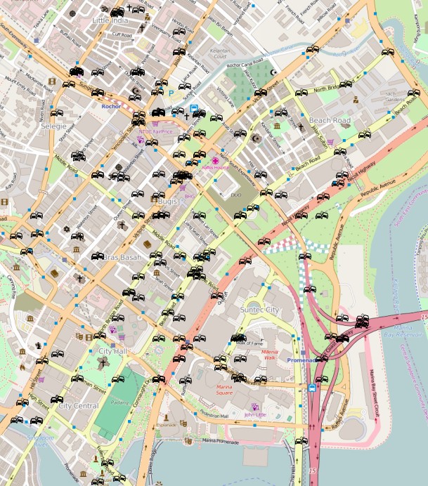
Spatial Point Patterns in Real World
Distribution of car collisions.
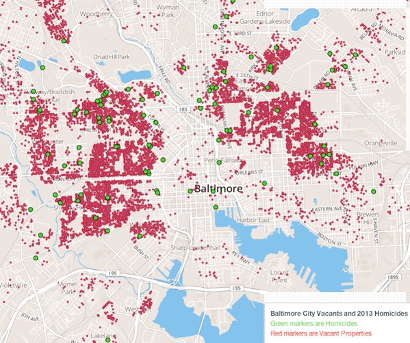
Spatial Point Patterns in Real World
Distribution of crime incidents.
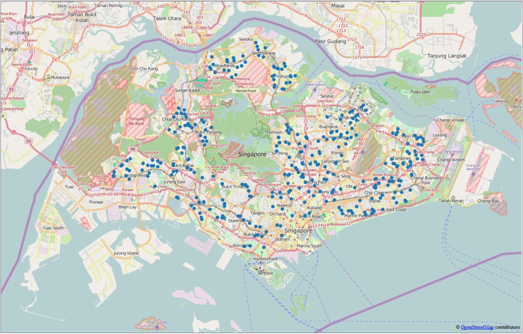
Spatial Point Patterns in Real World
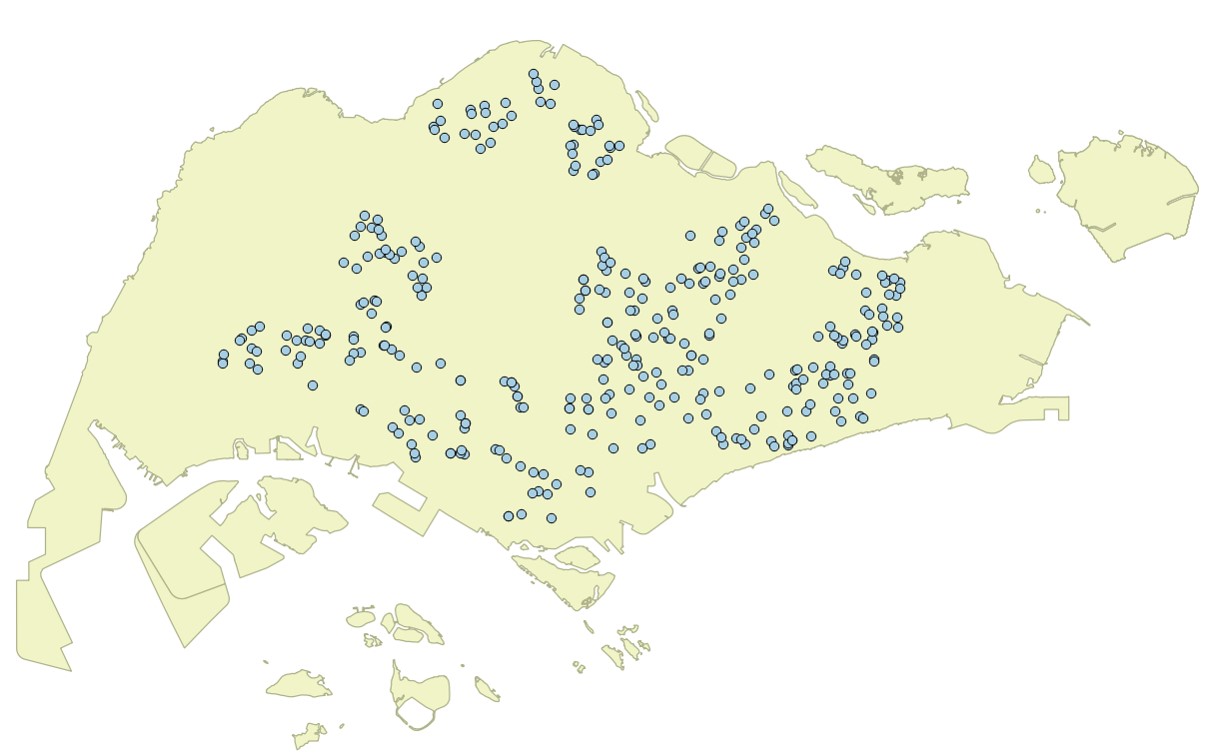
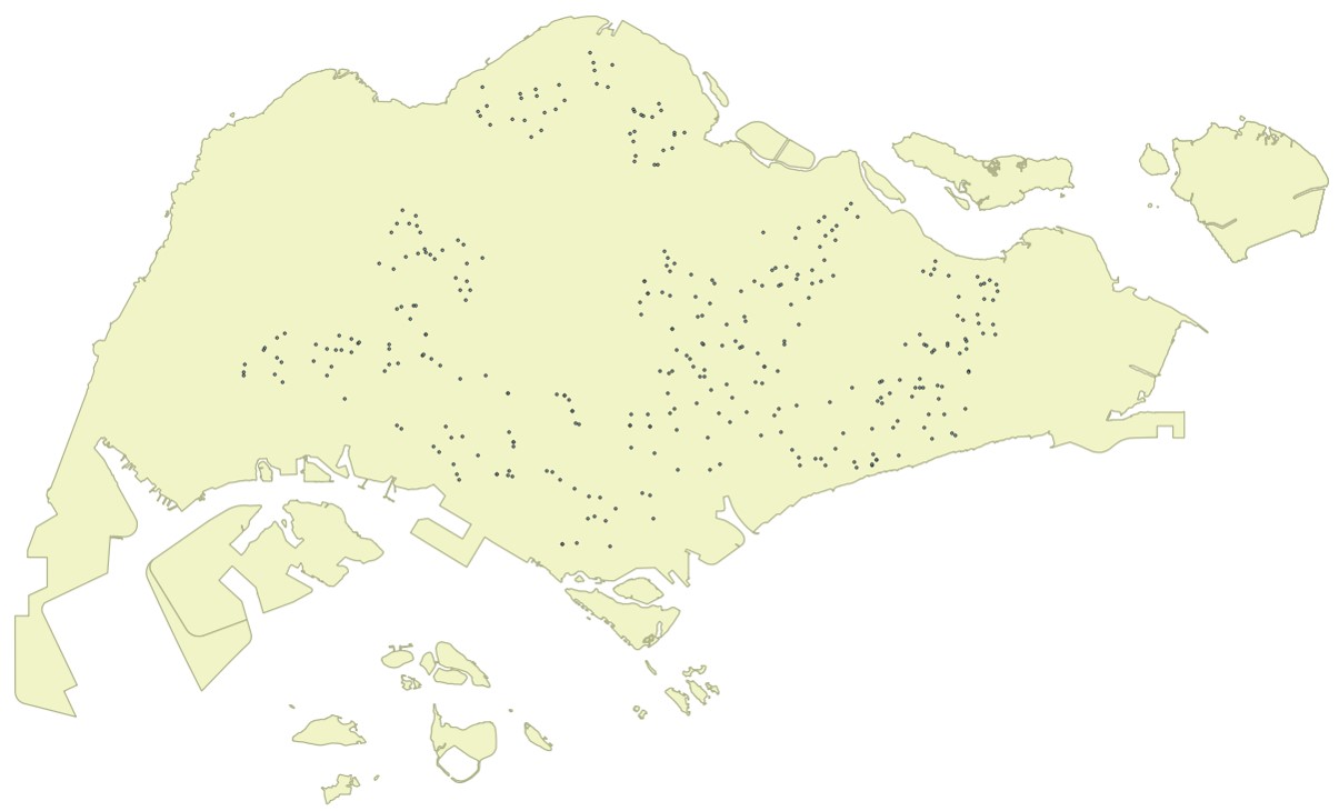
Distribution of public services such as education institutions.
Spatial Point Patterns in Real World
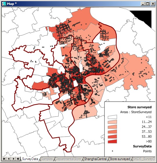
Locations of the different channel stores.
Spatial Point Patterns in Real World
Distribution of social media data such as tweets.
Real World Question
Location only
are points randomly located or patterned
Location and value
marked point pattern
is combination of location and value random or patterned
What is the underlying process?
Points on a Plane
Classic point pattern analysis
points on an isotropic plane
no effect of translation and rotation
classic examples: tree seedlings, rocks, etc
Distance
straight line only
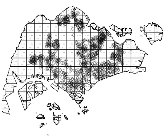
Real world spatial point patterns
Is this a random distribution?
Real world spatial point patterns
Is this a random distribution?
Spatial Point Patterns Analysis
Point pattern analysis (PPA) is the study of the spatial arrangements of points in (usually 2-dimensional) space.
The simplest formulation is a set X = {x ∈ D} where D, which can be called the study region, is a subset of Rn, a n-dimensional Euclidean space.
A fundamental problem of PPA is inferring whether a given arrangement is merely random or the result of some process.
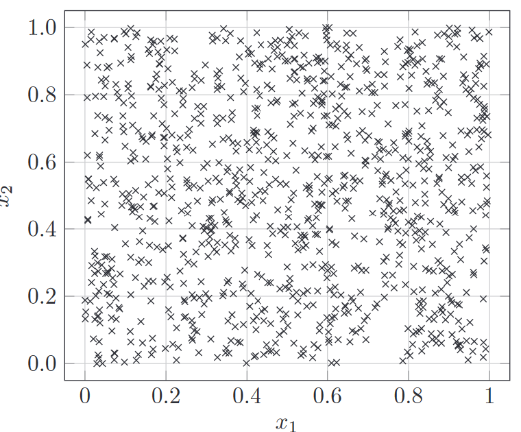
Homogeneous Spatial Point Patterns
A homogeneous spatial point pattern assumes that the points are distributed uniformly across the study area. The intensity (expected number of points per unit area) is constant throughout the region.
Characteristics:
The probability of observing a point is the same across the entire space.
The process generating the points does not depend on location.
The points are randomly and independently distributed across the space, leading to a uniform density.
Model:
Typically modeled by a Homogeneous Poisson Process, where the intensity λ (the number of points per unit area) is constant.
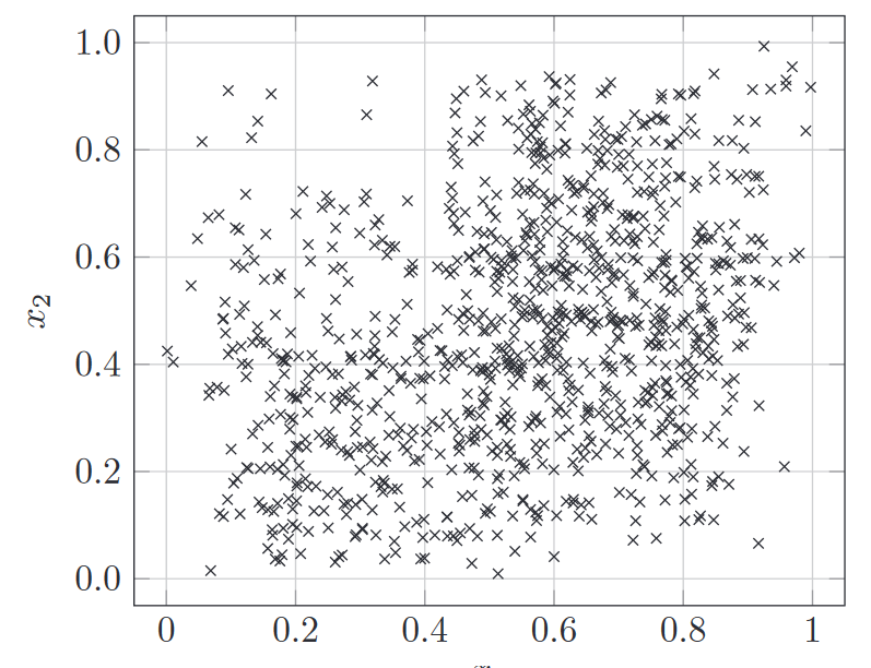
Heterogeneous Spatial Point Patterns
A heterogeneous spatial point pattern assumes that the intensity of points varies across the study area. The intensity function is not constant and may depend on spatial covariates, leading to non-uniform distribution.
Characteristics:
The probability of observing a point varies across the space, often depending on underlying factors like geography, environmental conditions, or other spatial variables.
The density of points can be higher in some regions and lower in others, leading to clusters or dispersed patterns.
Modeled by an Inhomogeneous Poisson Process (IPP), where the intensity function λ(x,y) varies with location. The intensity can be a function of spatial covariates or other influences.
Spatial Point Patterns Analysis Techniques
First-order vs Second-order Analysis of spatial point patterns.
First-order Spatial Point Patterns Analysis Techniques
Density-based
Kernel density estimation
Quadrat analysis,
Distance-based
Nearest Neighbour Index
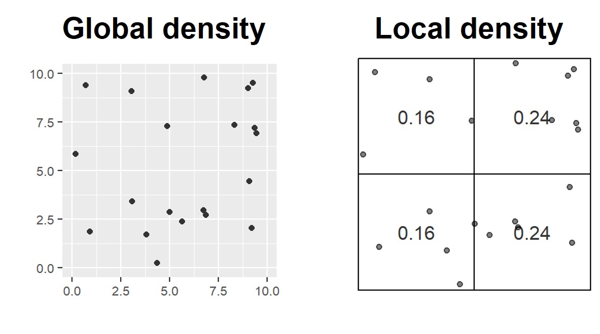
Basic concept of density-based measures
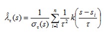
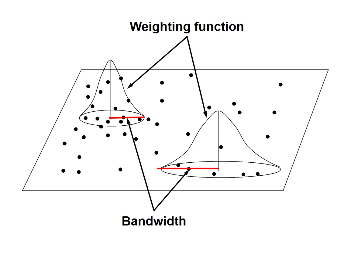
Kernel density estimation (Silverman 1986)
A method to compute the intensity of a point distribution.
The general formula:
Graphically
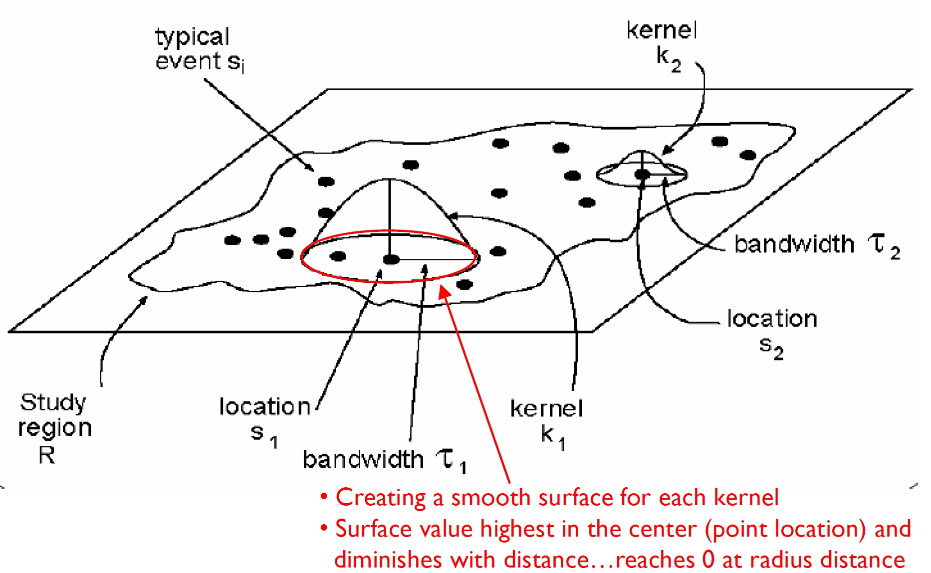
KDE Step 1: Computing point intensity
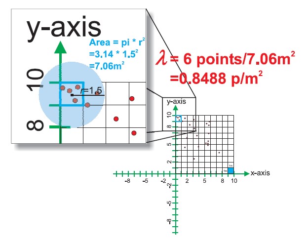
KDE Step 2: Spatial interpolation using kernel function
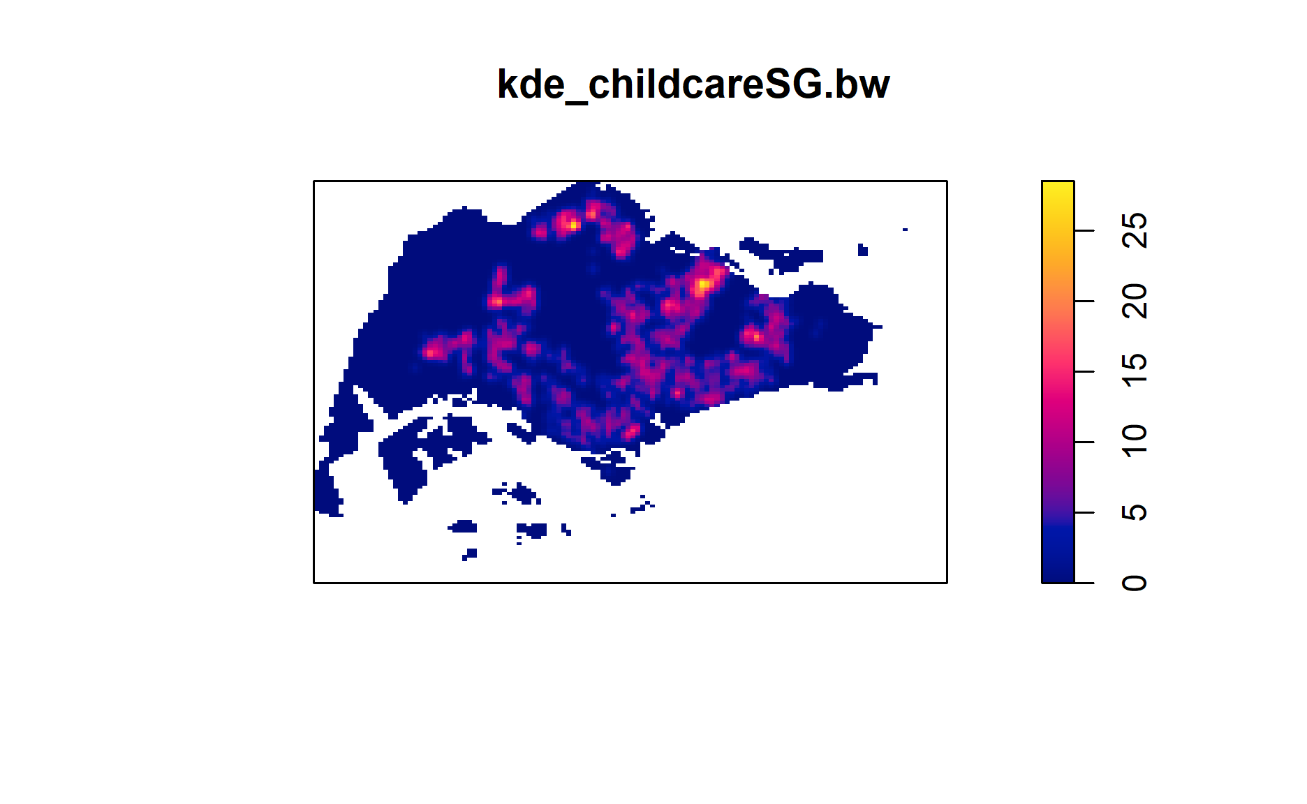
KDE Map of Childcare Services, Singapore
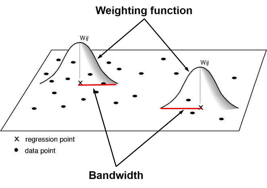
Adaptive Bandwidth
Adaptive schemes adjust itself according to the density of data: - Shorter bandwidths where data are dense and longer where sparse.
Finding nearest neighbors are one of the often used approaches.
Fixed bandwidth
Might produce large estimate variances where data are sparse, while mask subtle local variations where data are dense.
In extreme condition, fixed schemes might not be able to calibrate in local areas where data are too sparse to satisfy the calibration requirements (observations must be more than parameters).
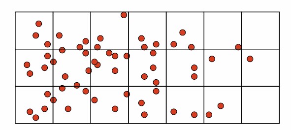
Quadrat Analysis – Step 1
Divide the study area into subregion of equal size,
often squares, but don’t have to be.
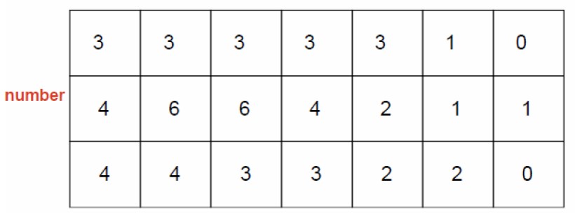
Quadrat Analysis – Step 2
Count the frequency of events in each region.
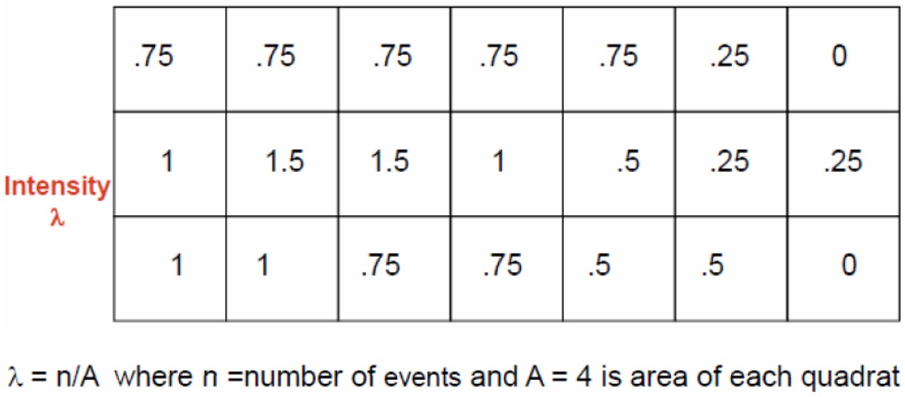
Quadrat Analysis – Step 3
Calculate the intensity of events in each region.
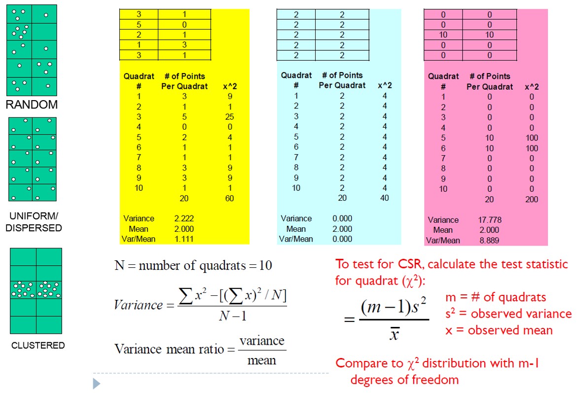
Quadrat Analysis – Step 4
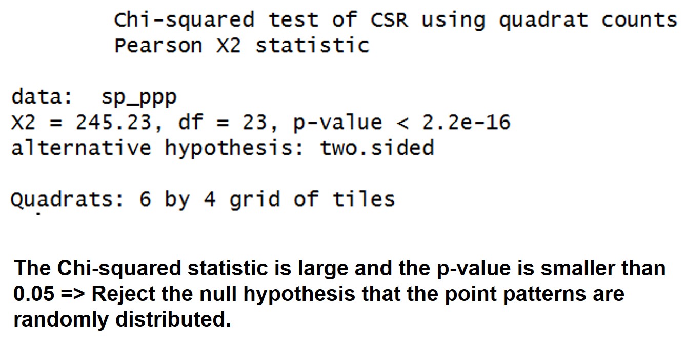
Calculate the quadrat statistics and perform CSR test.
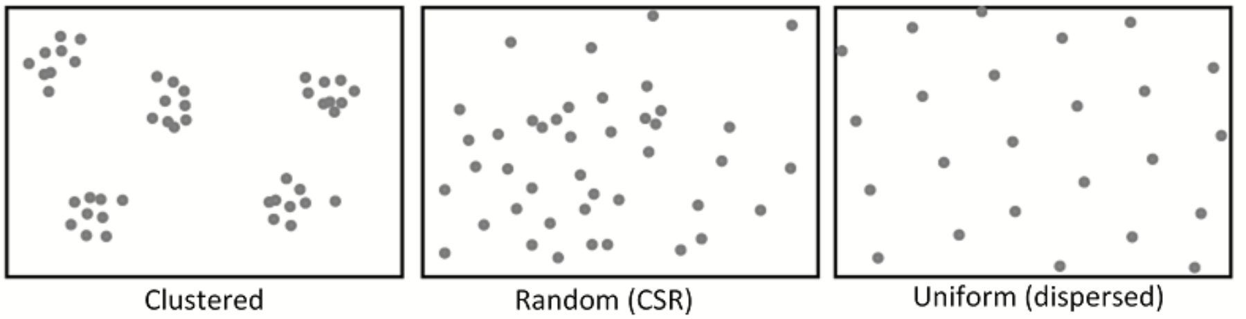
Quadrat Analysis – Variance-Mean Ratio (VMR)
For an uniform distribution, the variance is zero, - therefore, we expect a variance-mean ratio close to 0.
For a random distribution, the variance and mean are the same,
therefore, we expect a variance-mean ratio close to 1.
For a cluster distribution, the variance is relatively large,
therefore, we expect a variance-mean ratio greater than 1.]
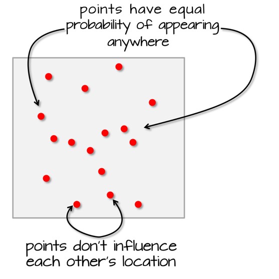
Complete Spatial Randomness (CSR)
CSR/IRP satisfy two conditions:
Any event has equal probability of being in any location, a 1st order effect.
The location of one event is independent of the location of another event, a 2nd order effect.
If the quadrat size is too small, they may contain only a couple of points, and
If the quadrat size is too large, they may contain too many points.
It is a measure of dispersion rather than a measure of pattern.
It results in a single measure for the entire distribution, so variation within the region are not recognised.
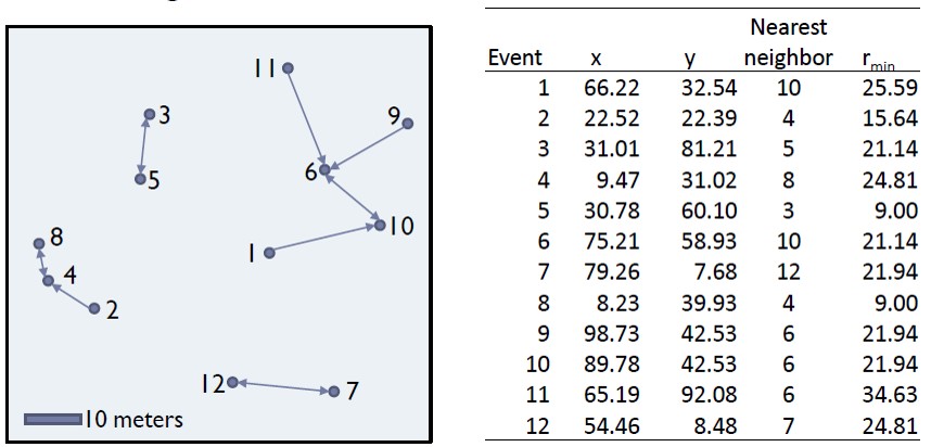
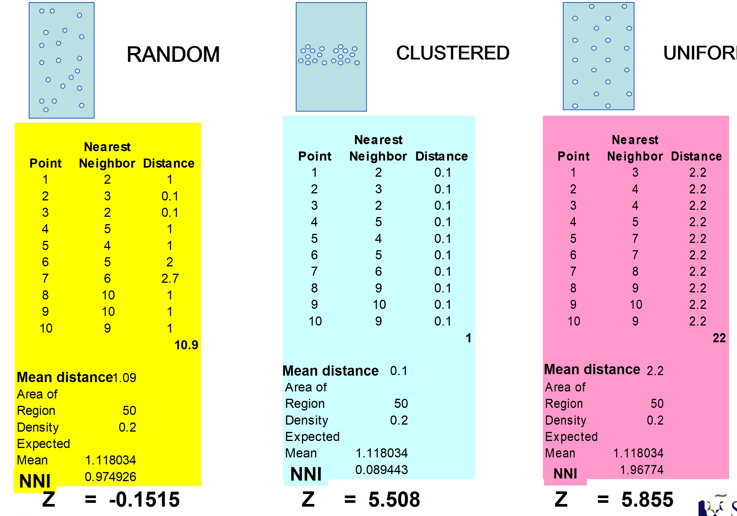
Distance-based: Nearest Neighbour Index
What is Nearest Neighbour?
Direct distance from a point to its nearest neighbour.
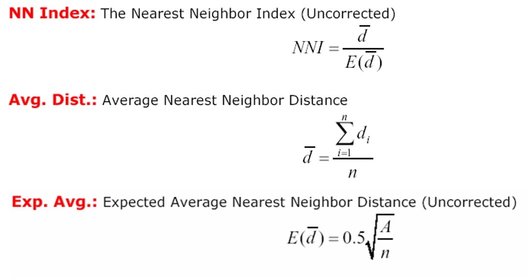
Nearest Neighbour Index
The Nearest Neighbour Index is expressed as the ratio of the Observed Mean Distance to the Expected Mean Distance.
Calculating Nearest Neighbour Index
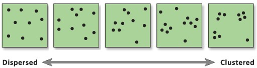
Interpreting Nearest Neighbour Index
The expected distance is the average distance between neighbours in a hypothetical random distribution.
If the index is less than 1, the pattern exhibits clustering,
If the index is equal to 1, the patterns exhibits random, and
If the index is greater than 1, the trend is toward dispersion or competition.
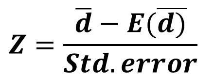
The test statistics
Null Hypothesis: Points are randomly distributed
Test statistics:
Reject the null hypothesis if the z-score is large and p-value is smaller than the alpha value.
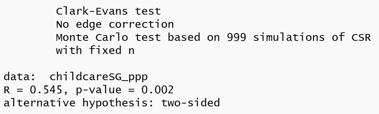
Interpreting Nearest Neighbour Index
The p-value is smaller than 0.05 => Reject the null hypothesis that the point patterns are randomly distributed.
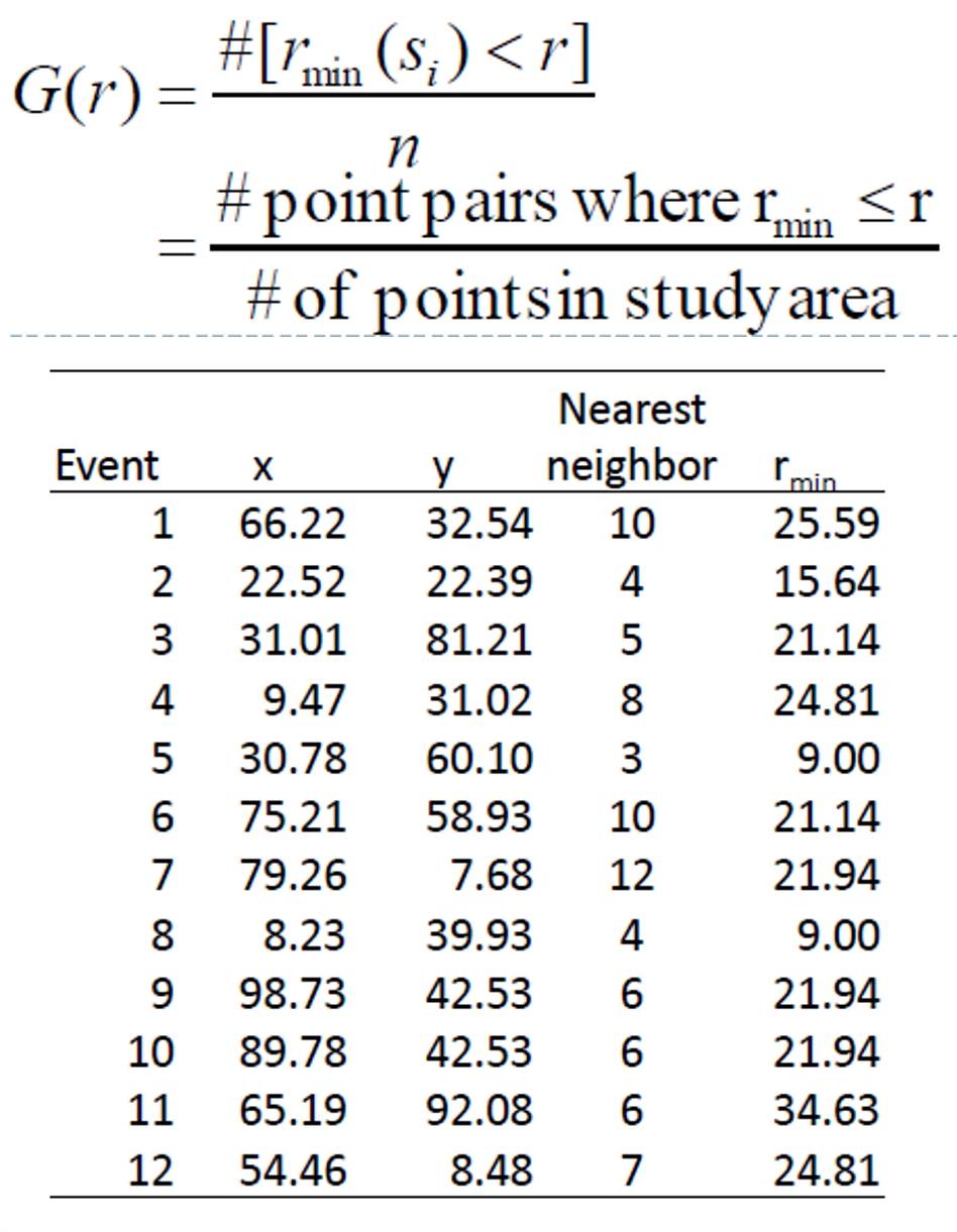
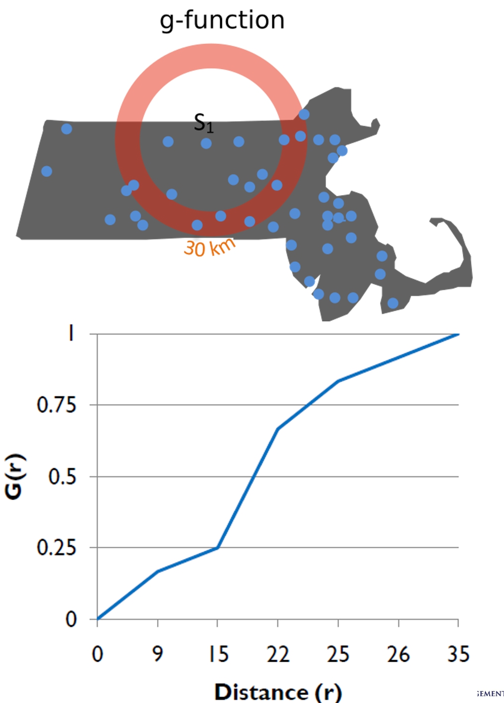
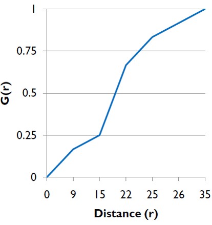
G function
The formula
Interpretation of G-function
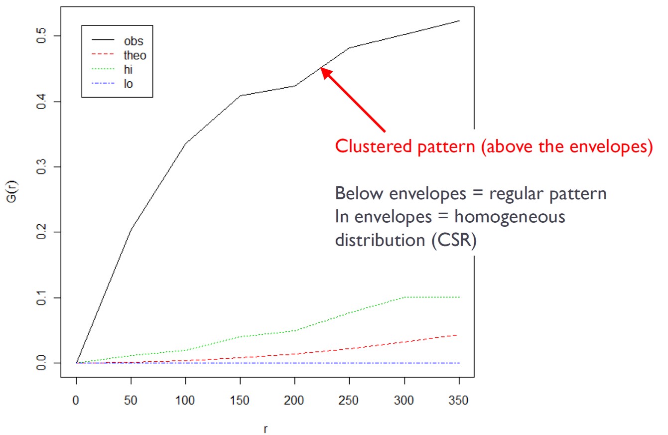
The shape of G-function tells us the way the events are spaced in a point pattern.
Clustered: G increases rapidly at short distance.
Evenness: G increases slowly up to distance where most events spaced, then increases rapidly.
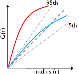
How do we tell if G is significant?
The significant of any departure from CSR (either cluster or regularity) can be evaluated using simulated “confidence envelopes”
Monte Carlo simulation test of CSR
Perform m independent simulation of n events (i.e. 999) in the study region.
For each simulated point pattern, estimate G(r) and use the maximum (95th) and minimum (5th) of these functions for the simulated patterns to define an upper and lower simulation envelope.
If the estimated G(r) lies above the upper envelope or below the lower envelope, the estimated G(r) is statistically significant.
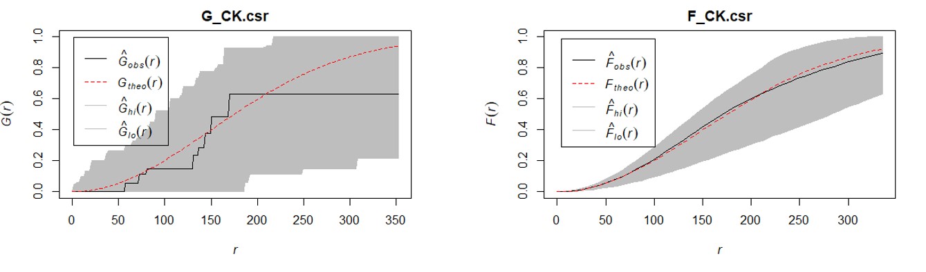
The significant test of G-function
F function
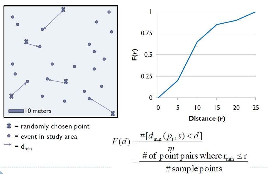
Select a sample of point locations anywhere in the study region at random
Determine minimum distance from each point to any event in the study area.
Three steps:
Randomly select m points (p1, p2, ….., pn),
Calculate dmin(pi,s) as the minimum distance from location pi to any event in the point patterns, and
Calculate F(d).
The F function formula
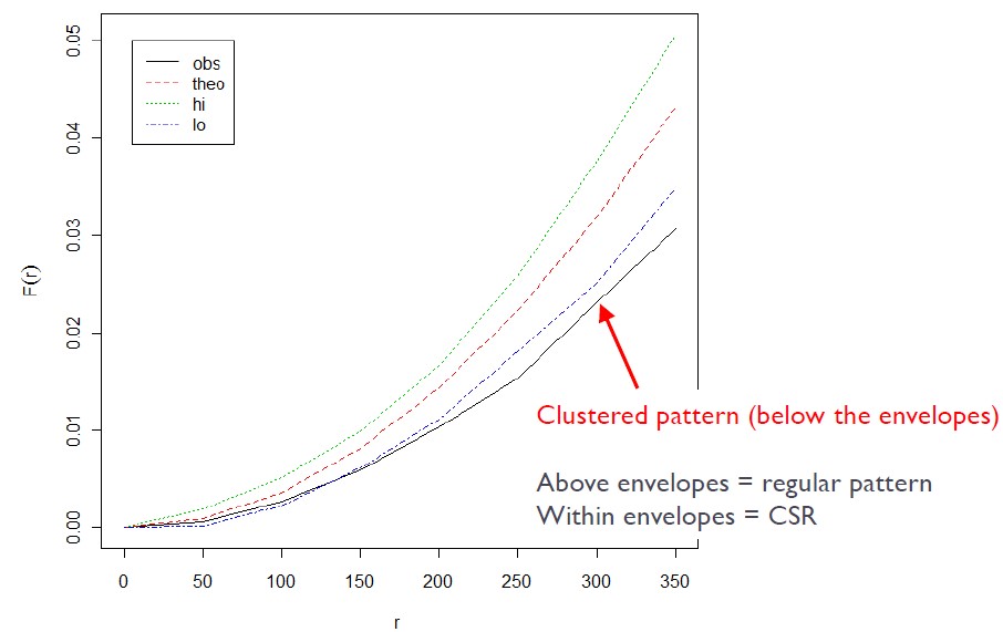
Interpretation of F-function
Clustered = F(r) rises slowly at first, but more rapidly at longer distances.
Evenness = F(r) rises rapidly at first, then slowly at longer distances.
The significant test of F-function
Comparison between G and F
Ripley’s K function (Ripley, 1981)
Limitation of nearest neighbor distance method is that it uses only nearest distance
Considers only the shortest scales of variation.
K function uses more points.
Provides an estimate of spatial dependence over a wider range of scales.
Based on all the distances between events in the study area.
Assumes isotropy over the region.
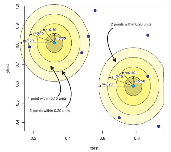
Calculating the K function
Construct a circle of radius h around each point event(i).
Count the number of other events (j) that fall inside this circle.
Repeat these two steps for all points (i) and sum results.
Increment h by a small amount and repeat the calculation.
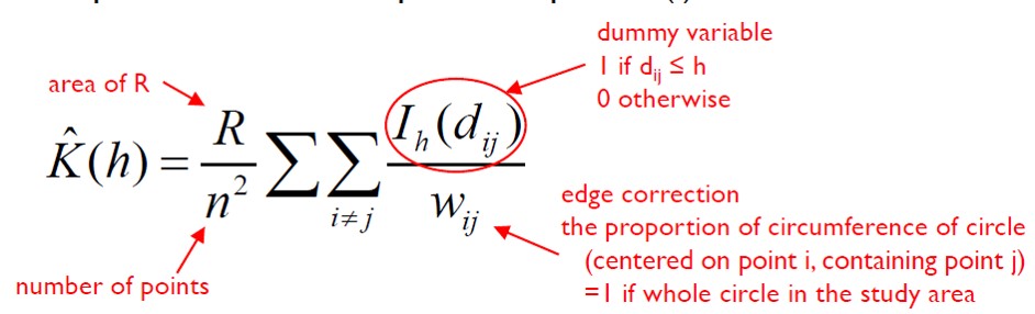
K function
The formula:
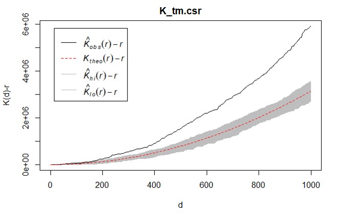
The K function complete spatial randomness test
K(h) can be plotted against different values of h.
But what should K look like for no spatial dependence?
Consider what K(h) should look like for a random point process (CSR)
The probability of an event at any point in R is independent of what other events have occurred and equally likely anywhere in R
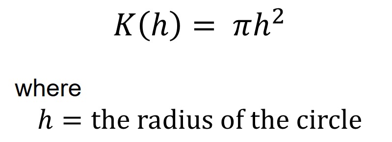
Interpreting the K function complete spatial randomness test
Under the assumption of CSR, the expected number of events within distance h of an event is:
Compare K(h) to 𝜋ℎ^2
K(h) < 𝜋ℎ^2 if point pattern is regular
K(h) > 𝜋ℎ^2 if point pattern is clustered
Above the envelop: significant cluster pattern
Below the envelop: significant regular
Inside the envelop: CSR
The L function (Besag 1977)
In practice, K function will be normalised to obtained a benchmark of zero.
The formula:
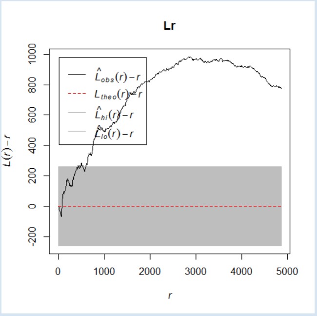
Interpreting the L function complete spatial randomness test
When an observed L value is greater than its corresponding L(theo)(i.e. red break line) value for a particular distance and above the upper confidence envelop, spatial clustering for that distance is statistically significant (e.g. distance beyond C).
When an observed L value is greater than its corresponding L(theo) value for a particular distance and lower than the upper confidence envelop, spatial clustering for that distance is statistically NOT significant (e.g. distance between B and C).
When an observed L value is smaller than its corresponding L(theo) value for a particular distance and beyond the lower confidence envelop, spatial dispersion for that distance is statistically significant. - When an observed L value is smaller than its corresponding L(theo) value for a particular distance and within the lower confidence envelop, spatial dispersion for that distance is statistically NOT significant (e.g. distance between A and B).
The grey zone indicates the confident envelop (i.e. 95%).
The L function (Besag 1977)
The modified L function
L(r)>0 indicates that the observed distribution is geographically concentrated.
In spatial point pattern analysis, we usually test whether the observed pattern is consistent with some null model (e.g., Complete Spatial Randomness, CSR).
spatstat does this by simulating nsim realisations of the null model.
For each simulation, it computes the test statistic (e.g., K-function, L-function, G-function, etc.) and compares it with the observed data.
Role of nsim
nsim is the number of simulated patterns generated under the null hypothesis.
A higher nsim means more accurate estimation of the sampling distribution, and more precise p-values.
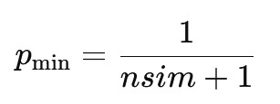
But p-values in Monte Carlo tests are discrete, and the smallest achievable p-value is
For example:
If nsim = 99, the smallest p-value you can report is 0.01.
If nsim = 999, the smallest possible p-value is 0.001.
So, larger nsim = finer resolution of p-values.
Confidence level and envelopes in spatstat
When you use envelope():
By default, you get pointwise simulation envelopes at a certain confidence level (e.g., 95%).
The confidence level is related to how wide the simulation band is. For a 95% envelope:
You drop the top 2.5% and bottom 2.5% of simulated values at each distance r.
The achievable confidence level is constrained by nsim:
For example, if nsim = 99, the finest possible two-tailed envelope is at 98% confidence (exclude the most extreme 1 value in each tail).
To get a “true” 95% envelope, you’d need nsim divisible appropriately (but spatstat interpolates when necessary).
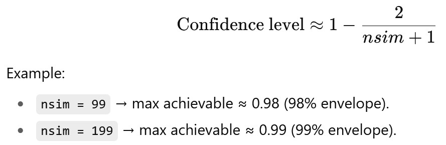
Confidence level and envelopes in spatstat
So the relationship is:
Rule of thumb in practice
Use at least nsim = 99 for quick tests, but prefer nsim = 999 or more if you want stable p-values and smooth envelopes.
Report p-values in terms of Monte Carlo resolution (e.g., “p < 0.05, based on 99 simulations” or “p < 0.001, based on 999 simulations”).