In-class Exercise 6: Take-Home Exercise 2 Kick Starter

Author

Affiliation

Dr. Kam Tin Seong
Assoc. Professor of Information Systems(Practice)

School of Computing and Information Systems,
Singapore Management University

Learning Outcome

By the end of this hands-on exercise, you will be able to:

• download dynamic data by using LTA DataMall API and postman;
• import and tidy geospatial data using sf and tidyverse;
• import and tidy aspatial data using tidyverse;
• create analytic hexagon data using sf;
• prepare

Loading the R package

The task

Write a code chunk to install and load tidyverse, sf, sfdep, tmap, knitr, kableExtra, and DT into R environment.

Note

• tidyverse, a family of modern R packages specially developed for performing data science tasks,
• sf, a modern R package specially developed for performing geospatial data science tasks except visualising geospatial data;
• tmap, an R package for create elegant thematic maps based on the principles of Layered Grammar of Graphics;
• knitr, an R package that provide an elegant, flexible, and fast static table generation with R;
• kableExtra, an extension of knitr for creating elegant html table with R; and
• DT, an R package DT provides an R interface to the JavaScript library DataTables for create interactive htnl tables.

The code

pacman::p_load(tidyverse, sf, sfdep, tmap, knitr, kableExtra, DT)

Extracting and Downloading Data Using LTA DataMall API

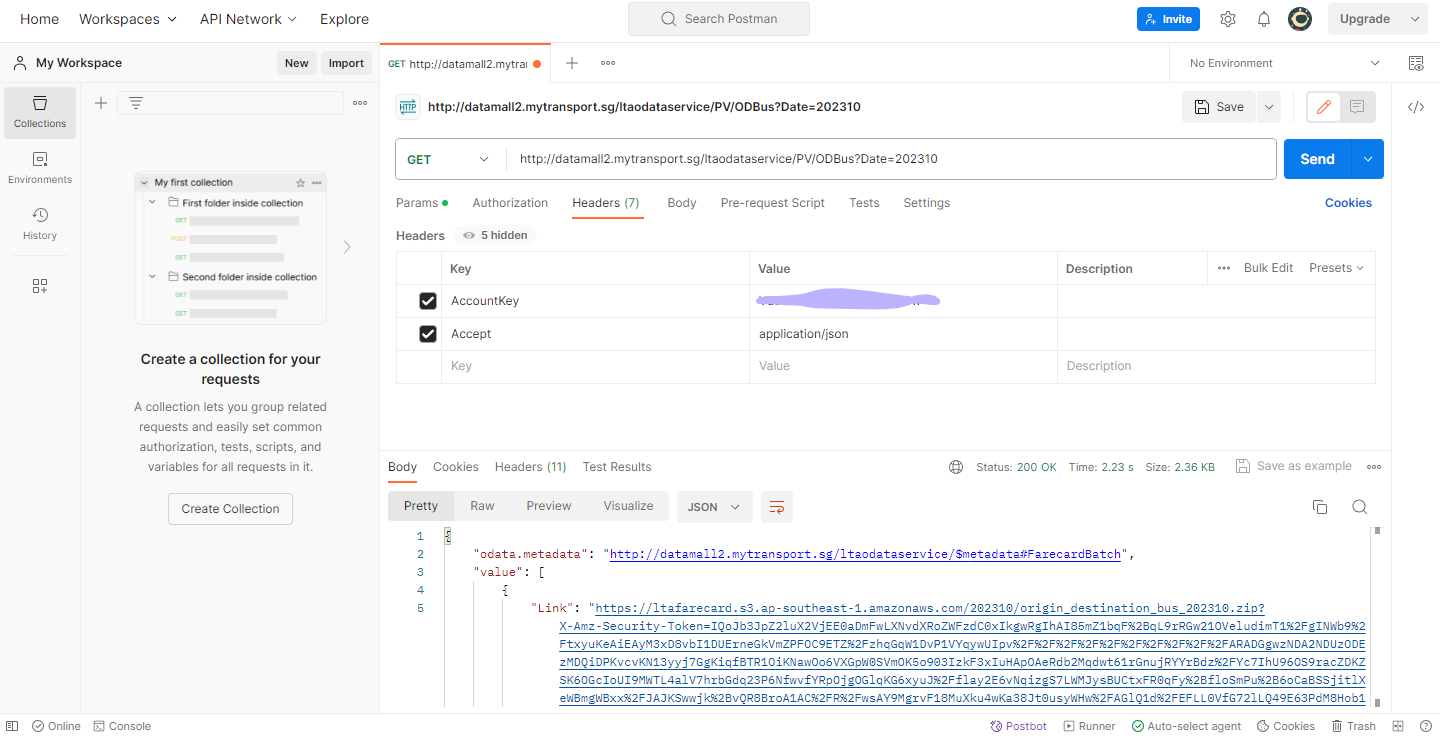
Follow the steps below to install postman desktop and make an API call.

---

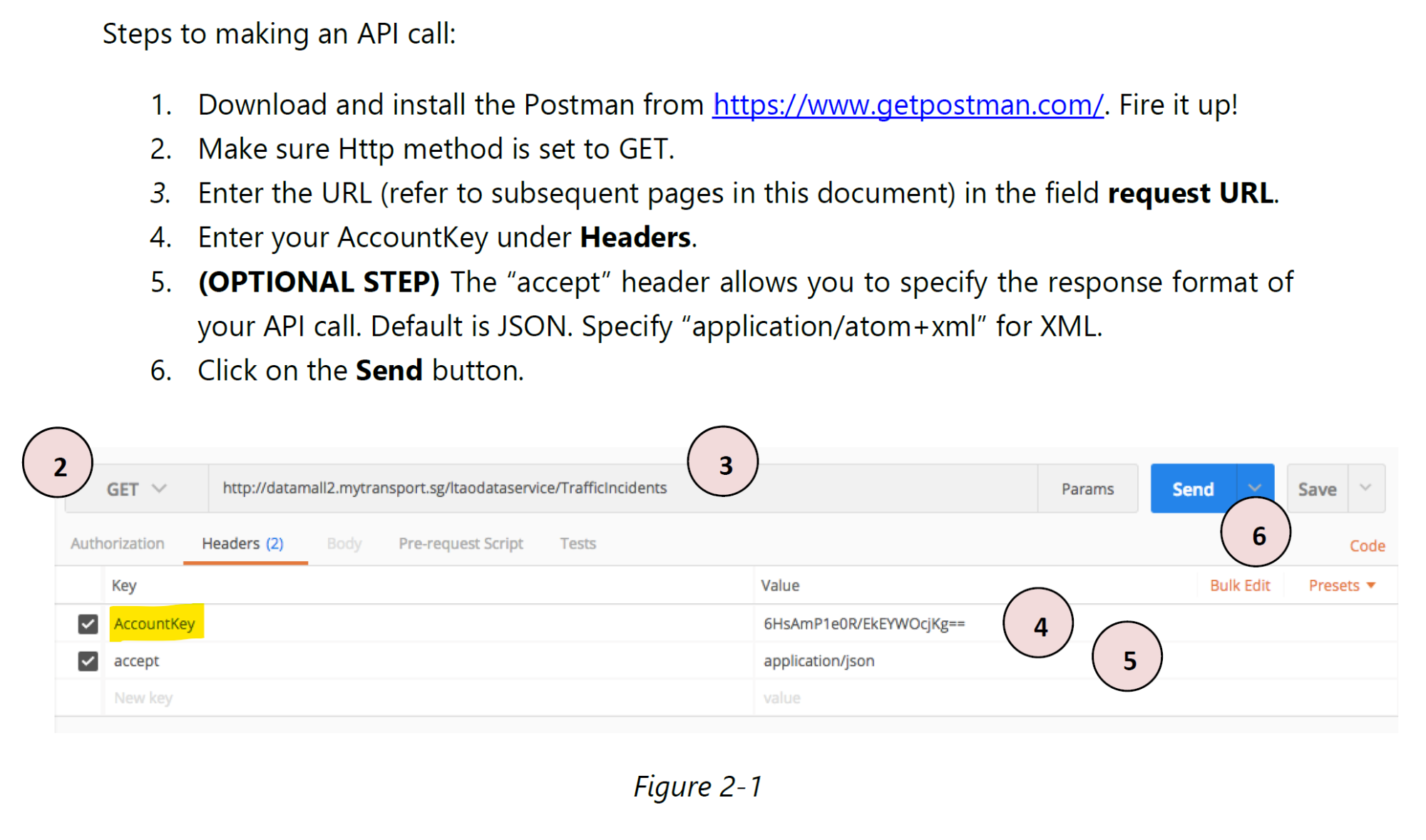
Downloading the dynamic data

Copy the url provide in line 5, must start from https:// onwards, then from the web browser, start a new page. Next, paste the url on the new page. The file will start download onto your computer.

Importing Data

The task

Write code chunks to perform the followings:

• Importing Bus Stop Location shapefile downloaded from LTA DataMall into R environment.
• Importing Master Plan 2019 Subzone Boundary (No Sea) from Singapore’s open data portal.
• Importing Passenger Volume by Origin Destination Bus Stops downloaded from LTA DataMall into R environment.

Bus Stop Location

BusStop = st_read(dsn = "data/LTADataMall/", 
                  layer = "BusStop") %>%
  st_transform(crs = 3414)

Reading layer `BusStop' from data source 
  `C:\tskam\ISSS626-AY2025-26Aug\In-class_Ex\In-class_Ex06\data\LTADataMall' 
  using driver `ESRI Shapefile'
Simple feature collection with 5172 features and 2 fields
Geometry type: POINT
Dimension:     XY
Bounding box:  xmin: 3970.122 ymin: 26482.1 xmax: 48285.52 ymax: 52983.82
Projected CRS: SVY21

Master Plan 2019 Subzone

mpsz = read_rds("data/rds/mpsz_sf.rds")

Note

Refer to 2.3.2 Importing Geospatial Data into R of R for Geospatial Data Science and Analytics to learn how to import and tidy a kml file.

O-D Bus Trips

odbus <- read_csv("data/LTADataMall/origin_destination_bus_202508.csv")

Note

read_csv() of readr package should be used instead of read.csv() of of Base R.

---

Visualising the geospatial data

Important

When working with geospatial data, it is highly recommended to visualise the geospatial data by using appropriate thematic mapping method(s).

Note

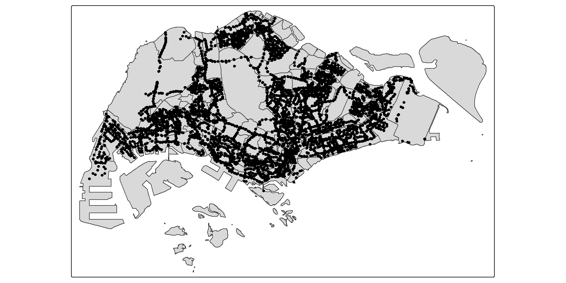
Actually, those bus stops are located along the Singapore-Johor Bahru causeway.

Figure below reveals that there a several bus stops (i.e black dots appear at the upper left) located outside of the main Singapore boundary.

---

Extracting Bus Stops located within Singapore

The code

In the code chunk below, st_join() of sf package is used to select all bus stops located within Singapore main island.

BusStop_in_SG <- st_join(
  BusStop, mpsz, 
  join = st_within, 
  left = FALSE)

Tip

Refer to st_join() to learn more about st_join() and other related functions.

The plot

Figure below reveals that all bus stops located outside of Singapore main island have been excluded.

Question:

Do you know how many bus stops are located outside of Singapore main island? Describe how the answer was derives.

Analytical Hexagon

Why Analytical Grids?

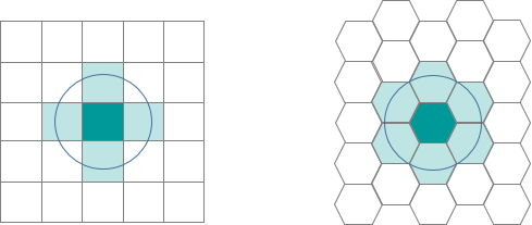
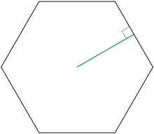
In geospatial analysis, regularly shaped grids are used for many reasons such as normalizing geography for mapping or to mitigate the issues of using irregularly shaped polygons created arbitrarily (such as county boundaries or block groups that have been created from a political process). Regularly shaped grids can only be comprised of equilateral triangles, squares, or hexagons, as these three polygon shapes are the only three that can tessellate (repeating the same shape over and over again, edge to edge, to cover an area without gaps or overlaps) to create an evenly spaced grid.

Why hexagon?

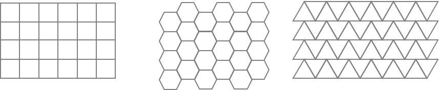
Hexagons reduce sampling bias due to edge effects of the grid shape, this is related to the low perimeter-to-area ratio of the shape of the hexagon. A circle has the lowest ratio but cannot tessellate to form a continuous grid. Hexagons are the most circular-shaped polygon that can tessellate to form an evenly spaced grid.

Deriving Analytical Hexagon

The task

Create analytics hexagon layer cover the entire Singapore.

The code

In the code chunk below, st_make_grid() of sf package is used to create the hexagon data set.

Important

It is high-recommended to read the reference guide of st_make_grid() to understand the usage of it.

hexagon <- st_make_grid(mpsz, 
                        cellsize = 700,
                        what = "polygon",
                        square = FALSE) %>%
  st_sf()

Warning

The output of st_make_grid() is an object of class sfc (simple feature geometry list column) with, depending on what and square, square or hexagonal polygons, corner points of these polygons, or center points of these polygons. Hence, st_sf() is needed to covert it to simple polygon feature data frame.

---

Checking the hexagon layer visually

Tip

Similarly, it is highly recommended to display the newly derived hexagon data.

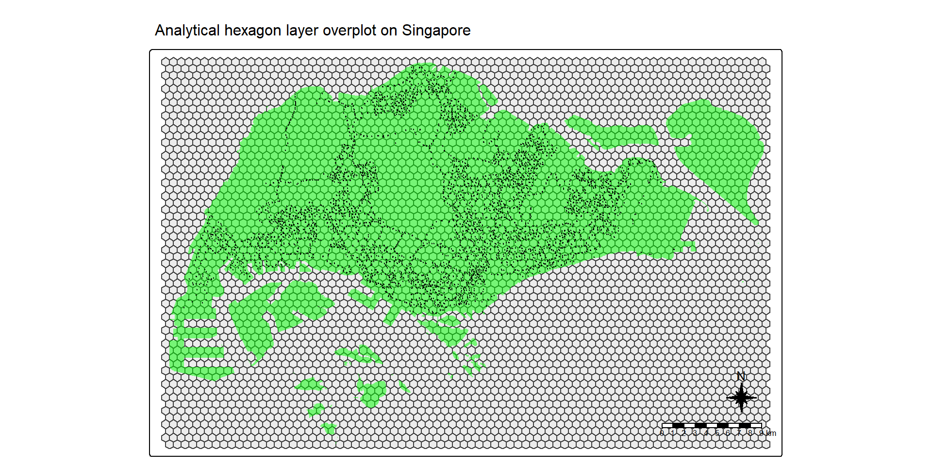
Figure above reveals that there are many hexagons without any bus stop in they. Some of them are located outside Singapore main island.

Selecting hexagons with bus stops

The code

Code chunk on the right eliminates hexagons without bus stop from the initial hexagon layer. It consists of three steps:

1. a new field called busstop_count is created.
2. st_intersects() is used to flag out bus stop located inside a hexagon. Then, length() is used to count the number of bus stops located inside a hexagon.
3. Lastly, filter() is used to select hexagons with at least one bus stop found.

hexagon$busstop_count =
  lengths(st_intersects(
    hexagon, BusStop_in_SG))

hexagon <- filter(
  hexagon, busstop_count > 0)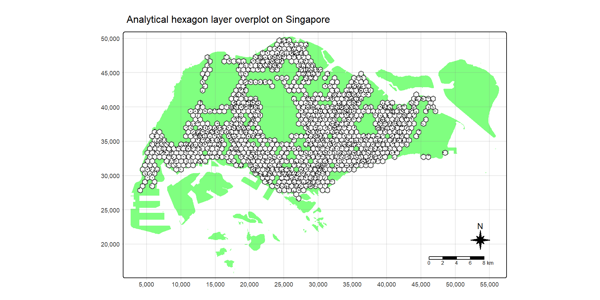

Checking the hexagon layer visually

Notice that only hexagons with bus stops remain.

---

Assigning ids to each hexagon

The issue

Let us examine the content of hexagon sf data frame below. Notice that the data frame does not include an ID field.

geometry	busstop_count
POLYGON ((4067.538 27468.93...	1
POLYGON ((4417.538 28075.15...	2
POLYGON ((4417.538 30500.02...	1
POLYGON ((4767.538 28681.37...	1
POLYGON ((4767.538 29893.8,...	4
POLYGON ((4767.538 31106.24...	1

The solution

hexagon <- hexagon %>% 
  select(, -busstop_count)

hexagon$HEX_ID <- sprintf(
  "H%04d", seq_len(
    nrow(hexagon))) %>% 
  as.factor()

Note

1. select() is used to drop busstop_count field from the sf data frame.
2. A new feld called HEX_ID is created. Then, sprintf(), seq_len() and nrow() are used to insert sequential ID values with a character H in front.
3. as.factor() is used to convert the values into factor data type.

Note

Notice that a new ID column called HEX_ID has been added into hexagon data frame and the values are 5-digit running number start with the letter H. At the same time, busstop_count field has been dropped from the data frame.

geometry	HEX_ID
POLYGON ((4067.538 27468.93...	H0001
POLYGON ((4417.538 28075.15...	H0002
POLYGON ((4417.538 30500.02...	H0003
POLYGON ((4767.538 28681.37...	H0004
POLYGON ((4767.538 29893.8,...	H0005
POLYGON ((4767.538 31106.24...	H0006

Preparing Trip Generation Data

Cleaning the data

The task

Before going deep in the wrangling, we will clean up the data so that we are left with a lightweight data set that R can process more easily.

1. We will retain and rename columns below to make them more understandable and easier to join with other data sets.
2. We will also rename the columns to make them more understandable and will make joining with other data sets easier.
3. Lastly, will also convert BUS_STOP_N to factor as it has a finite set of values so we can convert it to categorical data to make it easier to work with.

The code

trips <- odbus %>%
  select(c(ORIGIN_PT_CODE, DAY_TYPE, TIME_PER_HOUR, TOTAL_TRIPS)) %>%
  rename(BUS_STOP_N = ORIGIN_PT_CODE) %>%
  rename(HOUR_OF_DAY = TIME_PER_HOUR) %>%
  rename(TRIPS = TOTAL_TRIPS)
trips$BUS_STOP_N <- as.factor(trips$BUS_STOP_N)

The tidied sf data frame

BUS_STOP_N	DAY_TYPE	HOUR_OF_DAY	TRIPS
84671	WEEKENDS/HOLIDAY	9	3
10099	WEEKENDS/HOLIDAY	13	31
64601	WEEKENDS/HOLIDAY	21	3
53009	WEEKENDS/HOLIDAY	16	10
80051	WEEKENDS/HOLIDAY	18	4
70031	WEEKDAY	14	1

---

Populating Hexagon IDs into BusStop data frame

The task

Before we can aggregate trips generate at bus stops onto hexagon level, we need to populate the hexagon ids in hexagon data frame into BusStop data frame.

bs_hex <- st_intersection(
  BusStop, hexagon) %>%
  st_drop_geometry() %>%
  select(c(BUS_STOP_N, HEX_ID))

The bs_hex data frame

	BUS_STOP_N	HEX_ID
3092	25059	H0001
2439	25751	H0002
2554	25761	H0002
241	26379	H0003
2652	25741	H0004
1635	26399	H0005

---

Adding HEX_ID into bus trips data

The task and code chunk

To derive the hourly number of bus trips per hexagon, we need to add HEX_ID to trips data. By doing so, we will be able to aswer location questions such as how many bus trip originate from a certain hexagon?

In the code chunk below inner_join() is used to join the trips data with bs_hex.

trips <- inner_join(trips, bs_hex)

The revised trips data frame

BUS_STOP_N	DAY_TYPE	HOUR_OF_DAY	TRIPS	HEX_ID
84671	WEEKENDS/HOLIDAY	9	3	H0842
10099	WEEKENDS/HOLIDAY	13	31	H0424
64601	WEEKENDS/HOLIDAY	21	3	H0700
53009	WEEKENDS/HOLIDAY	16	10	H0564
80051	WEEKENDS/HOLIDAY	18	4	H0665
70031	WEEKDAY	14	1	H0678

---

Aggregating TRIPS based on HEX_ID

The code

In the code chunk below, group_by() and summarise() is used to aggregate TRIPS by HEX_ID, DAY_TYPE and HOUR_OF_DAY.

trips <- trips %>%
  group_by(
    HEX_ID,
    DAY_TYPE,
    HOUR_OF_DAY) %>%
  summarise(TRIPS = sum(TRIPS))

The trips data frame

The revised trip data frame should look similar to the table below.